SUBSCRIBE


Stormwater accumulation is a common challenge in developed environments, where infrastructure and impervious surfaces have altered natural drainage patterns. Elements such as roads, sidewalks, parking lots and buildings prevent rainfall from infiltrating the ground, thereby increasing surface runoff and causing unpredictable water pooling.
Even minor variations in surface elevation introduce unpredictable factors in determining how surface runoff converges1. Left unaddressed, these drainage issues can lead to hardscape and foundation damage, severe soil erosion, waterlogging and potential legal disputes with neighboring property owners.
Traditional drainage assessments typically rely on reactive visual inspections — such as identifying indicator species, erosion channels or watermarks on hardscapes — which only highlight problems after the damage has occurred. Fortunately, recent advancements in unmanned aerial vehicle (UAV) technology offer new, proactive opportunities to analyze landscape features at incredibly high spatial resolutions2.
Drone-based photogrammetry enables users to generate detailed orthomosaic imagery and elevation models that capture subtle variations in terrain. These high-resolution models reveal micro-topographic features that dictate water movement, allowing professionals to detect problem areas that visual inspections might miss.
By integrating these datasets with Geographic Information Systems (GIS), practitioners can perform advanced hydrologic analyses to calculate slope, flow direction and flow accumulation3. This proactive approach allows landscapers and facility managers to identify and correct problematic drainage spots before they escalate into costly repairs.
The purpose of this study was to demonstrate the use of drone-based aerial imagery and GIS-based hydrologic analysis to identify drainage paths on a campus lawn at the College of Coastal Georgia in Brunswick, Ga. This article provides step-by-step instructions and practical results to help landscaping professionals easily incorporate this workflow into their routine operations.
Methodology
The core methodology employed in this study is Structure-from-Motion (SfM) photogrammetry, a technique that generates high-resolution 3D models from a series of overlapping 2D photographs. SfM is now integrated into many accessible software programs4.
The first step involves acquiring photographs of the target area from multiple angles. Once the images are loaded into the SfM software, the program scans each photo to find unique, high-contrast visual points, such as the corner of a roof, a distinct rock or a painted line on a road.
The software then matches these exact features across all overlapping images. Because the camera moves between shots, the perspective on those features changes from frame to frame. By analyzing exactly how those matched points shift visually across different camera angles, the SfM algorithm works backward to calculate the camera’s position and orientation for each frame. The result is a “3D point cloud” containing millions of data points that digitally replicate the physical environment.
Materials
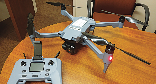
Theoretically, any drone with GPS capabilities can create a 3D model using SfM. For example, consumer models like the DJI Mini 5 Pro cost less than $1,000 as of earlier this year 2026. In this study, we used an ACSL Soten (Figure 1). Note: For commercial applications, operators must hold a drone pilot license (e.g., a Part 107 Remote Pilot Certificate in the U.S.) to perform flights legally.
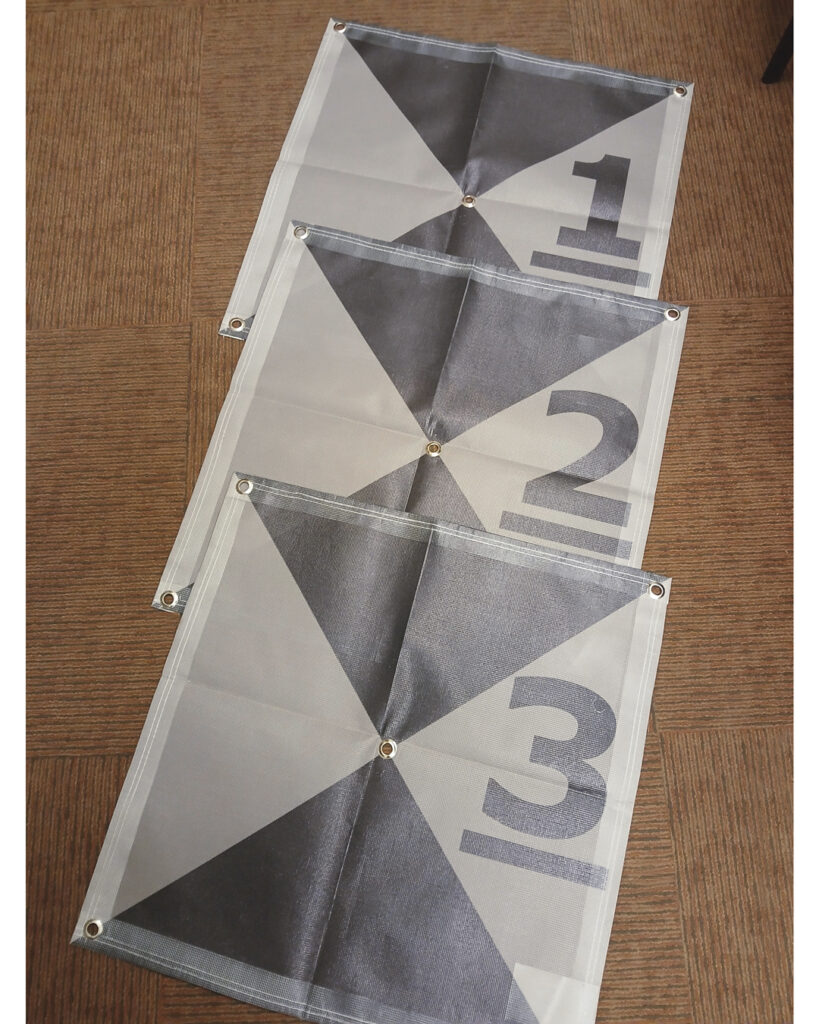
In addition to a drone, we highly recommend utilizing Ground Control Points (GCPs) (Figure 2) to increase the accuracy of the final model. GCPs can be as simple as flat pieces of paper or painted markers on the ground, provided they have no noticeable thickness profile.
While many commercial programs can process SfM, this demonstration utilizes the open-source software WebODM (webodm.org). We recommend downloading the installer version to simplify setup. Users will also need spatial analysis software, such as ArcGIS or QGIS, to analyze the resulting models.
Site description, next steps
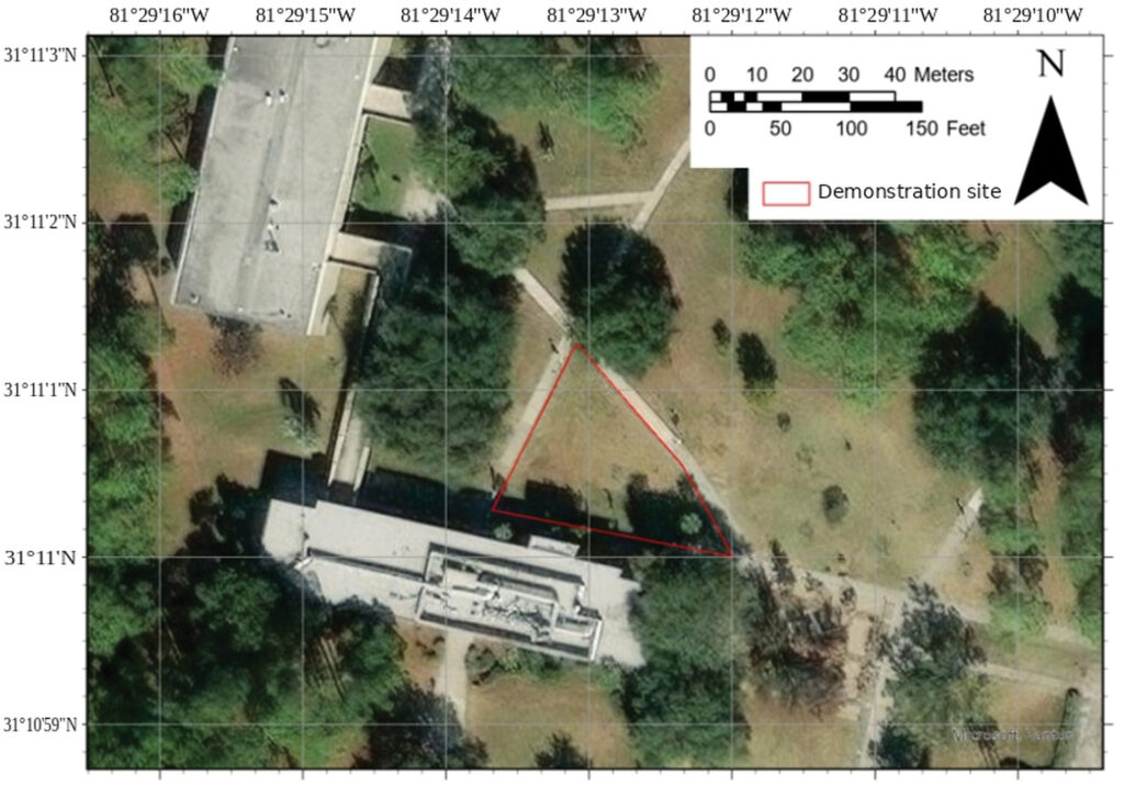
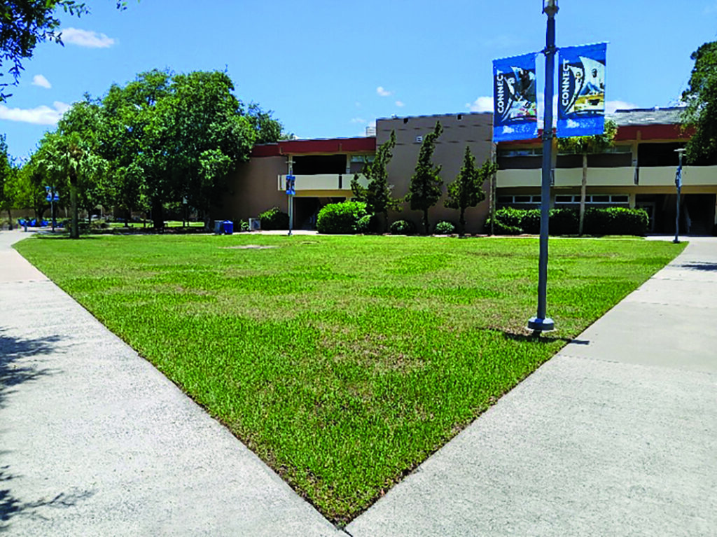
A medium-sized lawn (approximately 7,900 square feet) on the campus of the College of Coastal Georgia was used for the demonstration. An aerial view of the lawn is provided in Figure 3, and a ground-level photo taken on June 21, 2026, is provided in Figure 4. Note that the grass growth is spotty and non-uniform. Typically, such varied vegetation could mask true ground variations, making it an excellent test site for this methodology.
Once the site for this demonstration was established, the following steps were taken to acquire and analyze the images:
1. Create a flight plan. Automatic flight planning is available for many GPS-enabled drones, requiring the user to only set the overlap between adjacent images5. For this demonstration, we used a flight altitude of 100 feet and an air speed of 8 feet per second. The flight took about 10 minutes to finish.
2. Acquire aerial images. Lighting conditions should be consistent across the site, avoiding extreme contrasts. Details hidden in deep shadows might be lost, as consumer-grade cameras have limited dynamic range. GCPs should be deployed before the flight, both on the edges of and inside the area of interest. We recommend at least one GCP for every 6,400 square feet or one GCP every 80 feet6.
3. Collect GPS coordinates of GCPs. If a professional hand-held GPS receiver is unavailable, smartphone GPS apps can provide sufficient accuracy. Record the coordinates using the standard decimal longitude-latitude system.
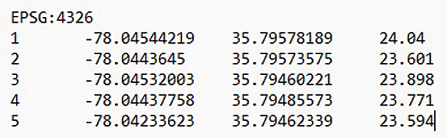
4. Create a “user GCP file” for WebODM. Using a simple text editor, create a file formatted like Figure 5. The first row, EPSG:4326, is the standard ID for the longitude-latitude system. Following this, each row contains the data for one GCP, separated by a “tab” space — GCP number, longitude, latitude and ground altitude (in meters). Remember: The western and southern hemispheres use negative numbers for longitude and latitude, respectively.
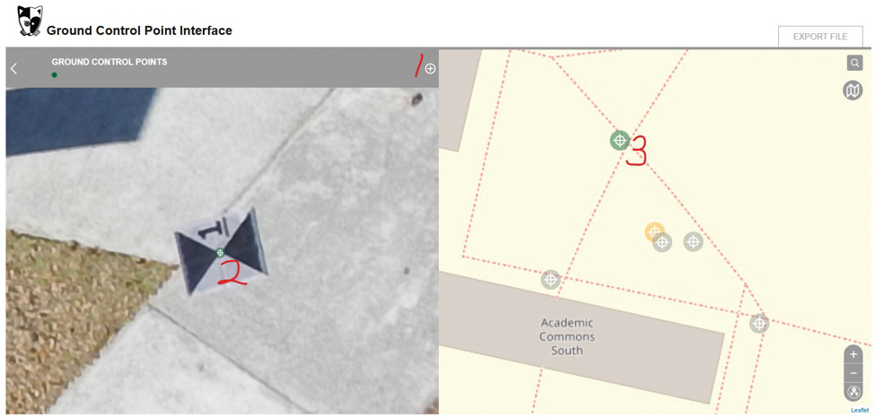
5. Mark out GCPs in the images. Launch WebODM and open the “GCP Interface.” Load the user GCP file that was just created, then upload the drone images. Double-click each image to enlarge it. When a GCP is spotted in the photo, click the plus sign (step 1 in Figure 6), then click the center of the photo (left-hand side of the screen, step 2 in Figure 6) and link it to the corresponding GCP on the right-hand side of the screen (step 3 in Figure 6). Repeat this for all images. Once finished, export this as the “linked GCP file.”
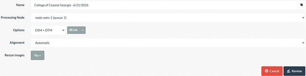
6. Run the SfM algorithm. Return to the WebODM dashboard. Click “Select Images and GCP” to upload the photos and the linked GCP file. Under “Options,” select “DSM+DTM,” then click “Review” (Figure 7)7. All the options will be locked, and the “Review” button will turn to “Start Processing.” Click it to run the SfM algorithm.
7. Download terrain models. Once processed, download the “Terrain Model.” A surface model depicts the topmost elevations (like grass and buildings), while a terrain model (DTM) depicts the bare ground beneath. To achieve this, WebODM uses a mathematical algorithm called the Simple Morphological Filters (SMRF) to strip away vegetation and derive accurate bare-ground elevations3. SMRF leverages the high resolution of the drone imagery — less than 1 centimeter per pixel in this study — to identify and link exposed ground pixels into a smooth terrain map.
8. Calculate flow direction. We now move to GIS spatial analysis software (ArcGIS Pro in this demonstration) to identify major flow paths. Before calculating flow accumulation, we must determine the flow direction at each grid cell. Use the “flow direction” geoprocessing tool, input the newly generated terrain model and run the tool.
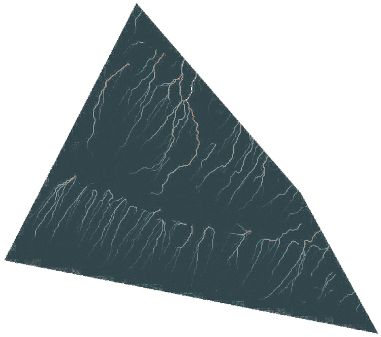
9. Calculate flow accumulation. Next, search for the “flow accumulation” geoprocessing tool. Input the flow direction raster we just created. The resulting output will resemble Figure 8, where the brightness of a cell represents the volume of water converging upon it.
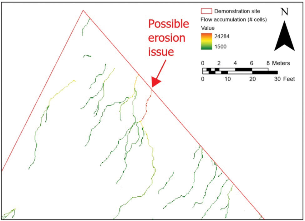
10. Isolate major flow paths. To make the map readable, we need to eliminate cells with negligible water accumulation. Use the “Raster Calculator” tool and input a simple logical statement using the SetNull command (Figure 9) to delete cells with values below a specific threshold (e.g., 1,500) from the file (“0621flowaccum.tif” in this demonstration). The final result (Figure 10) highlights only the primary drainage paths. The effluent path indicated by the red arrow in Figure 10 reveals a major point of flow accumulation where maintenance teams should proactively monitor for erosion.
Discussions and conclusions
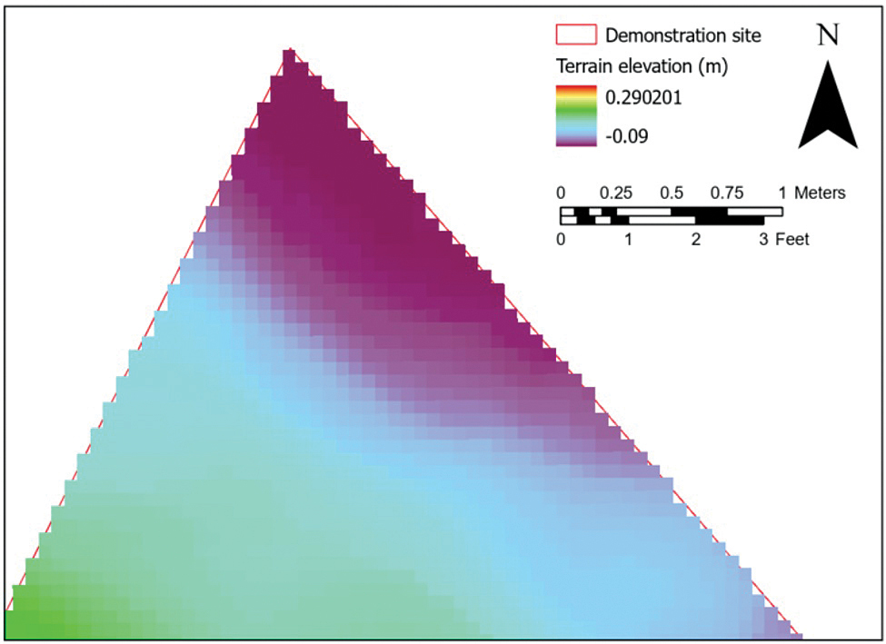
The workflow for creating a terrain model using SfM is highly effective for modern landscape management and hydrologic assessment. As demonstrated in Figure 11, the resulting Digital Terrain Model (DTM) is remarkably robust against variable vegetation heights, successfully stripping away spotty grass growth (Figure 4) to reveal the true ground elevation beneath.
The entire system setup is incredibly economical. The primary unavoidable expense is the drone itself, which can be acquired for under $1,000, while the processing and analysis can be completed using entirely open-source software (such as WebODM and QGIS)8.
Despite the low initial investment, the spatial resolution of the drone imagery is outstanding, yielding pixels smaller than 1 centimeter. This high level of detail is exactly what allows algorithms to effectively strip away the vegetation layer and isolate true ground variations.
Drones excel at scale2. A drone can survey a multi-acre landscaping site in less than an hour. In this demonstration, the aerial survey took about 10 minutes by a single worker. On the other hand, traditional methods are highly labor-intensive. Depending on the size and complexity of the site, it generally requires hours, if not days, from several skilled surveyors.
It is important to note that this methodology does not completely replace traditional surveying. Without an expensive airborne lidar system, optical drone imagery cannot penetrate thick, dense tree canopies9. For heavily wooded jobsites, traditional manual surveys remain necessary.
However, for open landscaping projects without significant canopy cover, this drone-to-GIS workflow provides a highly accurate, labor-saving and cost-effective method to proactively manage surface water and terrain variations in landscaping projects.
References
1. Hearn Landscape. (2026). How Overlooked Elevation Changes Create Ongoing Landscape Maintenance Problems. https://hearnlandscape.com/how-overlooked-elevation-changes-create-ongoing-landscape-maintenance-problems/
2. GIM International. (2020). UAV Photogrammetry as an Alternative to Classic Terrestrial Surveying Techniques. https://www.gim-international.com/content/news/uav-photogrammetry-as-an-alternative-to-classic-terrestrial-surveying-techniques
3. Akella, M. (2026). Hydrological mapping: Key methods and use cases. https://felt.com/blog/hydrological-mapping
4. Schwind, M., Starek, M. (2017). Producing High-quality 3D Point Clouds from Structure-from-Motion Photogrammetry. https://www.gim-international.com/content/article/structure-from-motion-photogrammetry
5. Lim, V. (2026). Sfm in Computer Vision: A Comprehensive Guide for 2025. https://www.shadecoder.com/topics/sfm-in-computer-vision-a-comprehensive-guide-for-2025
6. SkyeBrowse. (2026). Ground Control Points: The Complete Guide for Drone Mapping. https://www.skyebrowse.com/news/posts/ground-control-points-guide
7. WebODM. (2026). Creating Digital Elevation Models. https://docs.webodm.org/tutorials/creating-digital-elevation-models/
8. SkyeBrowse. (2026). Free Drone Mapping Software: Best Options Compared in 2026. https://www.skyebrowse.com/news/posts/free-drone-mapping-software
9. Alavi, H. (2026). Photogrammetry vs. LiDAR accuracy in RTK drone mapping. https://blog.emlid.com/photogrammetry-vs-lidar-accuracy-in-rtk-drone-mapping/